WAVE MOTION AND INTRODUCTION TO ELECTROMAGNETIC WAVES

 IN THE FOLLOWING CONTENT YOU MAY GET INSIGHT INTO THE AMAZING WORLD OF WAVES WHICH WE ARE COMPLETELY SURROUNDED BY.

LETS START THE JOURNEY ......

     A wave is a disturbance in a medium that carries energy without a net movement of particles. It may take the form of elastic deformation, a variation of pressure, electric or magnetic intensity, electric potential, or temperature.

PROPERTIES OF WAVES:-

• Transfers energy.
• Usually involves a periodic, repetitive Movement.
• Does not result in a net movement of the medium or particles in the medium (mechanical wave). 

TYPES OF WAVES:-

1)Mechanical waves

• Transverse Waves

Waves in which the medium moves at right angles to the direction of the wave.

Examples of transverse waves:

• Water waves (ripples of gravity waves, not sound through water)
• Light waves
• S-wave earthquake waves
• Stringed instruments
• Torsion wave

The high point of a transverse wave is a crest. The low part is a trough.

• Longitudinal Wave:

A longitudinal wave has the movement of the particles in the medium in the same dimension as the direction of movement of the wave.

Examples of longitudinal waves:

• Sound waves
• P-type earthquake waves
• Compression wave

Parts of longitudinal waves:

Compression: where the particles are close together.

Rarefaction: where the particles are spread apart.

2)Matter Waves:

Any moving object can be described as a wave When a stone is dropped into a pond, the water is disturbed from its equilibrium positions as the wave passes; it returns to its equilibrium position after the wave has passed.

3)Electromagnetic Waves:

These waves are the disturbance that does not need any object medium for propagation and can easily travel through the vacuum. They are produced due to various magnetic and electric fields. The periodic changes that take place in magnetic electric fields and therefore known as Electromagnetic Wave.

NOW WE WILL DISCUSS SOME MORE CONCEPTS RELATED TO THE WAVES:-

Wave equation in one space dimension

The wave equation is an important second-order linear partial differential equation for the description of waves—as they occur in classical physics—such as mechanical waves (e.g. water waves, sound waves and seismic waves) or light waves. It arises in fields like acoustics, electromagnetics, and fluid dynamics.

The wave equation in one space dimension can be written as follows:

${\displaystyle {\partial ^{2}u \over \partial t^{2}}=c^{2}{\partial ^{2}u \over \partial x^{2}}}$.

This equation is typically described as having only one space dimension x, because the only other independent variable is the time t. Nevertheless, the dependent variable u may represent a second space dimension, if, for example, the displacement u takes place in y-direction, as in the case of a string that is located in the x–y plane.

FOR COMPLETE DERIVATION OF ABOVE DESCRIBED EQUATION YOU MAY REFER TO THE FOLLOWING LINK :-

                                  COMPLETE DERIVATION OF WAVE EQUATION

Plane wave

 a plane wave is a special case of wave or field: a physical quantity whose value, at any moment, is constant over any plane that is perpendicular to a fixed direction in space.^[1]

For any position ${\displaystyle {\vec {x}}}$ in space and any time ${\displaystyle t}$, the value of such a field can be written as

${\displaystyle F({\vec {x}},t)=G({\vec {x}}\cdot {\vec {n}},t),}$

where ${\displaystyle {\vec {n}}}$ is a unit-length vector, and ${\displaystyle G(d,t)}$ is a function that gives the field's value as from only two real parameters: the time ${\displaystyle t}$, and the displacement ${\displaystyle d={\vec {x}}\cdot {\vec {n}}}$ of the point ${\displaystyle {\vec {x}}}$ along the direction ${\displaystyle {\vec {n}}}$. The latter is constant over each plane perpendicular to ${\displaystyle {\vec {n}}}$.

Traveling plane wave

The wavefronts of a plane wave traveling in 3-space

Often the term "plane wave" refers specifically to a traveling plane wave, whose evolution in time can be described as simple translation of the field at a constant wave speed ${\displaystyle c}$ along the direction perpendicular to the wavefronts. Such a field can be written as

${\displaystyle F({\vec {x}},t)=G\left({\vec {x}}\cdot {\vec {n}}-ct\right)\,}$

where ${\displaystyle G(u)}$ is now a function of a single real parameter ${\displaystyle u=d-ct}$, that describes the "profile" of the wave, namely the value of the field at time ${\displaystyle t=0}$, for each displacement ${\displaystyle d={\vec {x}}\cdot {\vec {n}}}$. In that case, ${\displaystyle {\vec {n}}}$ is called the direction of propagation. For each displacement ${\displaystyle d}$, the moving plane perpendicular to ${\displaystyle {\vec {n}}}$ at distance ${\displaystyle d+ct}$ from the origin is called a "wavefront". This plane travels along the direction of propagation ${\displaystyle {\vec {n}}}$ with velocity ${\displaystyle c}$; and the value of the field is then the same, and constant in time, at every one of its points.^[2]

Sinusoidal plane wave

The term is also used, even more specifically, to mean a "monochromatic" or sinusoidal plane wave: a travelling plane wave whose profile ${\displaystyle G(u)}$is a sinusoidal function. That is,

${\displaystyle F({\vec {x}},t)=A\sin \left(2\pi f({\vec {x}}\cdot {\vec {n}}-ct)+\varphi \right)\,}$

The parameter ${\displaystyle A}$, which may be a scalar or a vector, is called the amplitude of the wave; the scalar coefficient ${\displaystyle f}$ is its "spatial frequency"; and the scalar ${\displaystyle \varphi }$ is its "phase".

A true plane wave cannot physically exist, because it would have to fill all space. Nevertheless, the plane wave model is important and widely used in physics. The waves emitted by any source with finite extent into a large homogeneous region of space can be well approximated by plane waves when viewed over any part of that region that is sufficiently small compared to its distance from the source. That is the case, for example, of the light waves from a distant star that arrive at a telescope.

Plane standing wave

A standing wave is a field whose value can be expressed as the product of two functions, one depending only on position, the other only on time. A plane standing wave, in particular, can be expressed as

${\displaystyle F({\vec {x}},t)=G({\vec {x}}\cdot {\vec {n}})\,S(t)}$

where ${\displaystyle G}$ is a function of one scalar parameter (the displacement ${\displaystyle d={\vec {x}}\cdot {\vec {n}}}$) with scalar or vector values, and ${\displaystyle S}$ is a scalar function of time.

This representation is not unique, since the same field values are obtained if ${\displaystyle S}$ and ${\displaystyle G}$ are scaled by reciprocal factors. If ${\displaystyle |S(t)|}$ is bounded in the time interval of interest (which is usually the case in physical contexts), ${\displaystyle S}$ and ${\displaystyle G}$ can be scaled so that the maximum value of ${\displaystyle |S(t)|}$ is 1. Then ${\displaystyle |G({\vec {x}}\cdot {\vec {n}})|}$ will be the maximum field magnitude seen at the point ${\displaystyle {\vec {x}}}$.

PROPERTIES OF PLANE WAVES

A plane wave can be studied by ignoring the directions perpendicular to the direction vector ${\displaystyle {\vec {n}}}$; that is, by considering the function ${\displaystyle G(z,t)=F(z{\vec {n}},t)}$ as a wave in a one-dimensional medium.

Any local operator, linear or not, applied to a plane wave yields a plane wave. Any linear combination of plane waves with the same normal vector ${\displaystyle {\vec {n}}}$ is also a plane wave.

For a scalar plane wave in two or three dimensions, the gradient of the field is always collinear with the direction ${\displaystyle {\vec {n}}}$; specifically, ${\displaystyle \nabla F({\vec {x}},t)={\vec {n}}\partial _{1}G({\vec {x}}\cdot {\vec {n}},t)}$, where ${\displaystyle \partial _{1}G}$ is the partial derivative of ${\displaystyle G}$ with respect to the first argument.

The divergence of a vector-valued plane wave depends only on the projection of the vector ${\displaystyle G(d,t)}$ in the direction ${\displaystyle {\vec {n}}}$. Specifically,

${\displaystyle (\nabla \cdot F)({\vec {x}},t)\;=\;{\vec {n}}\cdot \partial _{1}G({\vec {x}}\cdot {\vec {n}},t)}$

In particular, a transverse planar wave satisfies ${\displaystyle \nabla \cdot F=0}$ for all ${\displaystyle {\vec {x}}}$ and ${\displaystyle t}$.

Phase velocity

The phase velocity of a wave is the rate at which the wave propagates in some medium. This is the velocity at which the phase of any one frequency component of the wave travels. For such a component, any given phase of the wave (for example, the crest) will appear to travel at the phase velocity.

The phase velocity is given in terms of the wavelength λ (lambda) and time period T as                  

Group velocity

The group velocity of a wave is the velocity with which the overall envelope shape of the wave's amplitudes—known as the modulation or envelope of the wave—propagates through space.

The group velocity v_g is defined by the equation:

${\displaystyle v_{g}\ \equiv \ {\frac {\partial \omega }{\partial k}}\,}$

where ω is the wave's angular frequency (usually expressed in radians per second), and k is the angular wavenumber (usually expressed in radians per meter). The phase velocity is: v_p = ω/k.

DERIVATION OF GROUP VELOCITY :- COMPLETE DERIVATION

This shows a wave with the group velocity and phase velocity going in different directions.^[1] The group velocity is positive (i.e., the envelope of the wave moves rightward), while the phase velocity is negative (i.e., the peaks and troughs move leftward).

Relation Between Group Velocity And Phase Velocity Equation

For the amplitude of wave packet let-

• ω is the angular velocity given by ω=2πf
• k is the angular wave number given by – k=2πλ
• t is time
• x be the position
• Vp phase velocity
• Vg be the group velocity

The phase velocity of a wave is given by the following equation:

vp=ωk…..(eqn 1)

Rewritting the above equation, we get:

ω=kvp…..(eqn 2)

Differentiating (eqn 2) w.r.t k we obtain,

dwdk=vp+kdvpdk…..(eqn 3)


As vg=dwdk, (eqn 3) reduces to:


vg=vp+kdvpdk

The above equation signifies the relationship between the phase velocity and the group velocity.

Hope you understood the relation between group velocity and phase velocity of a progressive wave.

Wavepackets and the Principle of Superposition

Wavepackets and the Principle of Superposition

To return momentarily to the electron traveling through a vacuum, it is clear physically that it must have a wave function that goes to zero far away in either direction (we’ll still work in one dimension, for simplicity). A localized wave function of this type is called a “wavepacket”. We shall discover that a wavepacket can be constructed by adding plane waves together. Now, the plane waves we add together will individually be solutions of the Schrödinger equation.

But does it follow that the sum of such solutions of the Schrödinger equation is itself a solution to the equation? The answer is yes—in other words, the Schrödinger equation

iℏ∂ψ(x,y,z,t)∂t=−ℏ22m∇2ψ(x,y,z,t)+V(x,y,z)ψ(x,y,z,t)

is a linear equation, that is to say, if ψ1(x,y,z,t), ψ2(x,y,z,t) are both solutions of the equation, then so is

ψ(x,y,z,t)=c1ψ1(x,y,z,t)+c2ψ2(x,y,z,t)

where c1 and c2 are arbitrary constants, as is easy to check. This is called the Principle of Superposition.

The essential point is that in Schrödinger’s equation every term contains a factor ψ, but no term contains a factor ψ2 (or a higher power). That’s what is meant by a “linear” equation. If the equation did contain a constant term, or a term including ψ2, superposition wouldn’t work—the sum of two solutions to the equation would not itself be a solution to the equation.

In fact, we have been assuming this linearity all along: when we analyze interference and diffraction of waves, we just add the two wave amplitudes at each spot. For the double slit, we take it that if the wave radiating from one slit satisfies the wave equation, then adding the two waves together will give a new wave which also satisfies the equation.

The First Step in Building a Wavepacket: Adding Two Sine Waves

If we add together two sine waves with frequencies close together, we get beats. This pattern can be viewed as a string of wavepackets, and is useful for gaining an understanding of why the electron speed calculated from λf=c above is apparently half what it should be.

We use the trigonometric addition formula:

sin((k−Δk)x−(ω−Δω)t)+sin((k+Δk)x−(ω+Δω)t)=2sin(kx−ωt)cos((Δk)x−(Δω)t)

This formula represents the phenomenon of beats between waves close in frequency. The first term, sin(kx−ωt), oscillates at the average of the two frequencies. It is modulated by the slowly varying second term, often called the “envelope function”, which oscillates once over a spatial extent of order π/Δk. This is the distance over which waves initially in phase at the origin become completely out of phase. Of course, going a further distance of order π/Δk, the waves will become synchronized again.

That is, beating two close frequencies together breaks up the continuous wave into a series of packets, the beats. To describe a single electron moving through space, we need a single packet. This can be achieved by superposing waves having a continuous distribution of wavelengths, or wave numbers within of order Δk, say, of k. In this case, the waves will be out of phase after a distance of order π/Δk but since they have many different wavelengths, they will never get back in phase again.

Electromagnetic waves can be imagined as a self-propagating transverse oscillating wave of electric and magnetic fields. This 3D animation shows a plane linearly polarized wave propagating from left to right. The electric and magnetic fields in such a wave are in-phase with each other, reaching minima and maxima together

The First Step in Building a Wavepacket: Adding Two Sine Waves

If we add together two sine waves with frequencies close together, we get beats. This pattern can be viewed as a string of wavepackets, and is useful for gaining an understanding of why the electron speed calculated from λf=c$\lambda f=c$ above is apparently half what it should be.

We use the trigonometric addition formula:

sin((k−Δk)x−(ω−Δω)t)+sin((k+Δk)x−(ω+Δω)t)=2sin(kx−ωt)cos((Δk)x−(Δω)t)sin⁡((k−Δk)x−(ω−Δω)t)+sin⁡((k+Δk)x−(ω+Δω)t)=2sin⁡(kx−ωt)cos⁡((Δk)x−(Δω)tThis formula represents the phenomenon of beats between waves close in frequency. The first term, 

This formula represents the phenomenon of beats between waves close in frequency. The first term, sin(kx−ωt)$\sin (kx-\omega t)$, oscillates at the average of the two frequencies. It is modulated by the slowly varying second term, often called the “envelope function”, which oscillates once over a spatial extent of order π/Δk$\pi /\mathrm{\Delta }k$. This is the distance over which waves initially in phase at the origin become completely out of phase. Of course, going a further distance of order π/Δk$\pi /\mathrm{\Delta }k$, the waves will become synchronized again.

That is, beating two close frequencies together breaks up the continuous wave into a series of packets, the beats. To describe a single electron moving through space, we need a single packet. This can be achieved by superposing waves having a continuous distribution of wavelengths, or wave numbers within of order Δk$\mathrm{\Delta }k$, say, of k$k$. In this case, the waves will be out of phase after a distance of order π/Δk$\pi /\mathrm{\Delta }k$ but since they have many different wavelengths, they will never get back in phase again.

ELECTROMAGNETIC WAVES:-

Electromagnetic waves are also known as EM waves that are produced when an electric field comes in contact with the magnetic field. It can also be said that electromagnetic waves are the composition of oscillating electric and magnetic fields. Electromagnetic waves are solutions of Maxwell’s equations, which are the fundamental equations of electrodynamics.

Electromagnetic waves are shown by a sinusoidal graph. It consists of time-varying electric and magnetic fields which are perpendicular to each other and are also perpendicular to the direction of propagation of waves. Electromagnetic waves are transverse in nature. The highest point of the wave is known as crest while the lowest point is known as a trough. In vacuum, the waves travel at a constant velocity of 3 x 108 m.s-1.

Electromagnetic Wave Equation

• Electromagnetic wave equation describes the propagation of electromagnetic waves in a vacuum or through a medium.
• The electromagnetic wave equation is a second order partial differential equation.
• It is a 3D form of the wave equation.
• The homogeneous form of the equation is written as,

(υ2ph▽2−∂2∂t2)E=0(υ2ph▽2−∂2∂t2)B=0

Where,υph=1μϵ√

Intensity of an Electromagnetic Wave

I=PA=12cϵ0E20=12cμ0B20

Speed of Electromagnetic Waves in Free Space

It is given by

C=1(μ0ϵ0)√

Where,

μ0 is called absolute permeability. It’s value is 1.257×10−6TmA−1

ϵ0 is called absolute permittivity. It’s value is 8.854×10−12C2N−1m−2

C is the velocity of light in vacuum = velocity of electromagnetic waves in free space = 3×108ms−1

Electromagnetic Spectrum

Maxwell's Equations

Maxwell's equations represent one of the most elegant and concise ways to state the fundamentals of electricity and magnetism. From them one can develop most of the working relationships in the field. Because of their concise statement, they embody a high level of mathematical sophistication and are therefore not generally introduced in an introductory treatment of the subject, except perhaps as summary relationships.

FOR COMPLETE DETAILS ABOUT MAXWELL'S EQUATION CLICK HERE

Energy & Momentum In Electromagnetic Waves

In a region of empty space where $\overrightarrow{E}$ and $\overrightarrow{B}$ fields are present, the total energy density $u$ is given by:

$$u=\frac{1}{2}{ϵ}_0{E}^2+\frac{1}{2{\mu }_0}{B}^2$$

For electromagnetic waves in a vacuum,

$$\begin{array}{cc}B& =\frac{E}{c}\\ & =\sqrt{{ϵ}_0{\mu }_0}E\end{array}$$

It follows that:

$$u={ϵ}_0{E}^2$$

In a vacuum, the energy density associated with the $\overrightarrow{E}$ field is equal to the energy of the $\overrightarrow{B}$ field.

In general, the energy density $u$ of an electromagnetic wave depends on position and time.

Electromagnetic waves transport energy from one region to another – they carry the energy density $u$ with them as they advance.

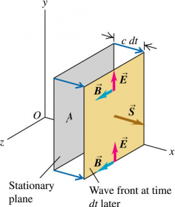
Consider a stationary plane, perpendicular to the x-axis, that coincides with the wave front at a certain time. In a time $dt$ after this, the wave front moves a distance $dx=cdt$ to the right of the plane.

Consider an area A on this stationary plane, the energy $dU$ in the space to the right of this area must have passed through the area to reach the new location.

Hence,

$$\begin{array}{cc}dU& =udV\\ & =\left({ϵ}_0{E}^2\right)\left(Acdt\right)\end{array}$$

The energy flow per unit time per unit area is given by:

$$\begin{array}{cc}S& =\frac{1}{A}\frac{dU}{dt}\\ & ={ϵ}_{0}c{E}^2\\ & ={ϵ}_0{c}^{2}E\left(\frac{1}{c}E\right)\\ & =\frac{1}{{\mu }_0}EB\end{array}$$

The energy flow per unit time per unit area has a term attached to it: Poynting vector, $\overrightarrow{S}$, where the direction is in the direction of propagation of the wave.

$$\begin{array}{cc}\overrightarrow{S}& =\frac{1}{{\mu }_0}\overrightarrow{E}\times \overrightarrow{B}\\ S& =\frac{1}{{\mu }_0}EB\end{array}$$

The total energy flow per unit time out of any closed surface is given by:

$$P=\oint \overrightarrow{S}.d\overrightarrow{A}$$

Let’s calculate the Poynting vector for typical sinusoidal waves:

$$\begin{array}{cc}\overrightarrow{E}(x,t)& =E_{\text{max}}\cos (kx-\omega t)\hat{j}\\ \overrightarrow{B}(x,t)& =B_{\text{max}}\cos (kx-\omega t)\hat{k}\end{array}$$

$$\begin{array}{cc}\overrightarrow{S}(x,t)& =\frac{1}{{\mu }_0}\overrightarrow{E}(x,t)\times \overrightarrow{B}(x,t)\\ & =\frac{1}{{\mu }_0}{E}_{\text{max}}{B}_{\text{max}}{\cos }^2(kx-\omega t)\hat{i}\\ & =\frac{1}{2{\mu }_0}{E}_{\text{max}}{B}_{\text{max}}[1+\cos 2(kx-\omega t)]\hat{i}\end{array}$$

The intensity of the radiation is the magnitude of the average value of the Poynting vector,

$$\begin{array}{cc}I& =S_{\text{average}}\\ & =\frac{E_{\text{max}}{B}_{\text{max}}}{2{\mu }_0}\\ & =\frac{1}{2{\mu }_{0}c}{E}_{max}^2\\ & =\frac{c}{2{\mu }_0{c}^2}{E}_{\text{max}}^2\\ & =\frac{1}{2}{ϵ}_{0}c{E}_{\text{max}}^2\\ & =\frac{1}{2}\sqrt{\frac{{ϵ}_0}{{\mu }_0}}{E}_{\text{max}}^2\end{array}$$

Electromagnetic waves also carry momentum $p$, with a corresponding momentum density. Let’s calculate the momentum carried by electromagnetic waves by using the well known relativistic formula: $E^2=p^2{c}^2+m^2{c}^4$. According to quantum mechanics, the electromagnetic radiation is made up of massless particles called photons, with momentum $p=\frac{E}{c}$ for individual photons.

It follows from $p=\frac{E}{c}$ that the momentum density for electromagnetic waves must be equal to the energy density divided by c. Since the energy density for electromagnetic waves is given by: $u={ϵ}_0{E}^2$

$$\begin{array}{cc}\frac{dp}{dV}& =\frac{{ϵ}_0{E}^2}{c}\\ & ={ϵ}_{0}EB\\ & =\frac{EB}{{\mu }_0{c}^2}\\ & =\frac{S}{c^2}\end{array}$$

We can further express the above as momentum transferred per unit time per unit area:

$$\begin{array}{cc}\frac{dp}{dV}& =\frac{S}{c^2}\\ \frac{dp}{Acdt}& =\frac{S}{c^2}\\ \frac{1}{A}\frac{dp}{dt}& =\frac{S}{c}\\ \frac{1}{A}\frac{dp}{dt}& =\frac{EB}{{\mu }_{0}c}\end{array}$$

This momentum is a property of the field – it is not associated with the mass of a moving particle in the usual sense. This momentum is responsible for the phenomenon of radiation pressure. If an electromagnetic wave with an average value of Poynting vector of $S_{\text{av}}$ is incident on an object, with no reflection and transmission, the radiation pressure on the object will be given by: (NOTE: $p_{\text{rad}}$ is radiation pressure and $dp$ is the infinitesimal change in momentum.)

$$\begin{array}{cc}{p}_{\text{rad}}& =\frac{F_{\text{rad}}}{A}\\ & =\frac{1}{A}\frac{dp}{dt}\\ & =\frac{S_{\text{av}}}{c}\\ & =\frac{I}{c}\end{array}$$

If all of the incident electromagnetic waves are reflected by the object, the resulting radiation pressure will be:

$$\begin{array}{cc}{p}_{\text{rad}}& =\frac{2S_{\text{av}}}{c}\\ & =\frac{2I}{c}\end{array}$$